When pricing a portfolio of trades, you need a curve group comprising curves that are needed to determine expected future cashflows (projection) and their present value (discounting).
To calibrate such curves against prevailing market data, you need to define:
- a curve configuration that holds the data provider mapping to the curve group
- a market data environment
- the applicable valuation settings
For illustration purposes, a generic curve calibration can be performed on a standalone basis at the curve configuration level, against a hypothetical portfolio of IRS, inflation and FX trades relevant to each curve in the curve group.
On this page, we will discuss how to:
We will also provide a detailed description of the curve calibration algorithm applied to minimise potential valuation errors.
We will also discuss the application of CSA discounting.
You can use the pre-configured ‘XPLAIN DEFAULT’, ‘LONDON’ curve configurations or the ‘NEW CURVE CONFIGURATION’ example that you may have defined.
Running a Generic Curve Calibration
Under
The curve calibration algorithm applied when performing a portfolio valuation will minimise the potential number of failed curve calibrations to ensure that the maximum number of trades can be valued.
Once you have run a curve calibration, you can export the calibration results.
| Field Name | Description | Permissible Values |
|---|---|---|
| Market Data Group | The market data group that contains the raw market data | See Market Data |
| Market Data Source | Data type (raw, preliminary cleansed or overlay) + Data provider (primary or secondary) |
RAW | PRELIMINARY | OVERLAY PRIMARY | SECONDARY See using MD exception management results |
| Stripping Type | Dual stripping (for the projection and discount curves) or Single curve stripping See here. |
OIS (DUAL) | SINGLE |
| Discount Ccy | Applicable single currency for discounting purposes or If Discount Ccy = 'Local Ccy', the discount currency will be a function of the trade type and user parameterisation (see here) |
Any permissible discount currency Local Ccy |
| Curve Date | The market data's historical curve date (default = system date) | YYYY-MM-DD (ISO 8601) |
| Valuation Date | The valuation date (default = Curve Date) | YYYY-MM-DD (ISO 8601) |
| Triangulation Ccy | The triangulation currency used first when no direct base vs counter curve can be found for foreign cashflow discounting | Any permissible discount currency |
| Bid/Mid/Ask | Market data side for projection and discounting curves, FX rates, ATM swaption and FX volatilities, and Swaption and FX volatility skews | Bid | Mid | Ask |
Curves/Curve Configurations/NEW CURVE CONFIGURATION
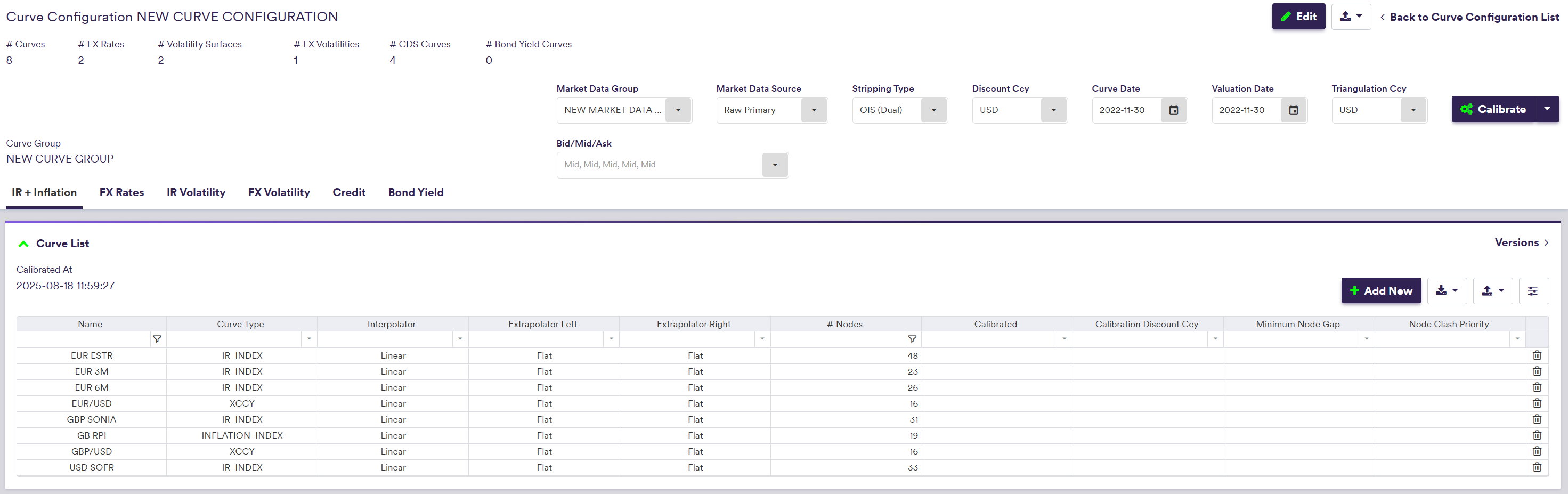
In this example, you will calibrate the ‘NEW CURVE CONFIGURATION’ with the following parameters:
- valuation date and curve date set to 30th November 2022
- market data from the existing ‘12PM LONDON’ market data group
- raw market data from the primary provider (meaning market data that have not been processed for anomaly detection)
- dual stripping type (OIS discounting)
- USD discount currency
- mid market data
Once the calibration has been performed, you can see which interest rate and inflation curves have been successfully calibrated and which curve will be used as the discount curve for a given currency.
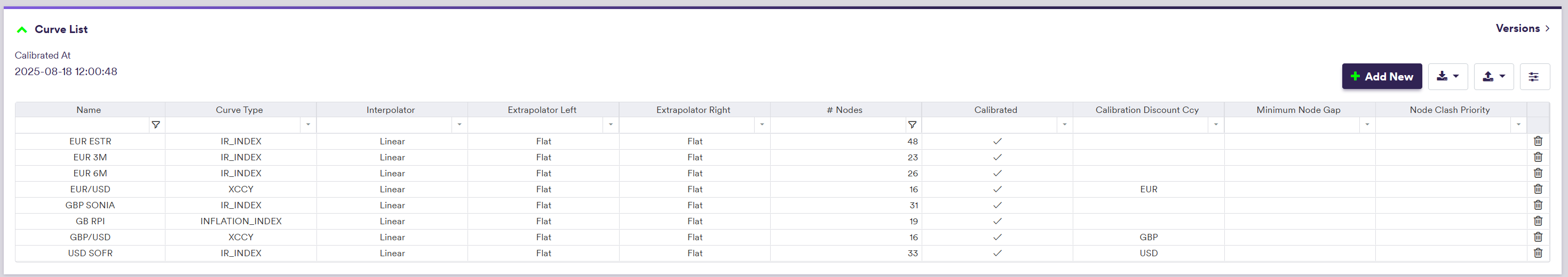
You can also export all calibration results at the curve configuration level.
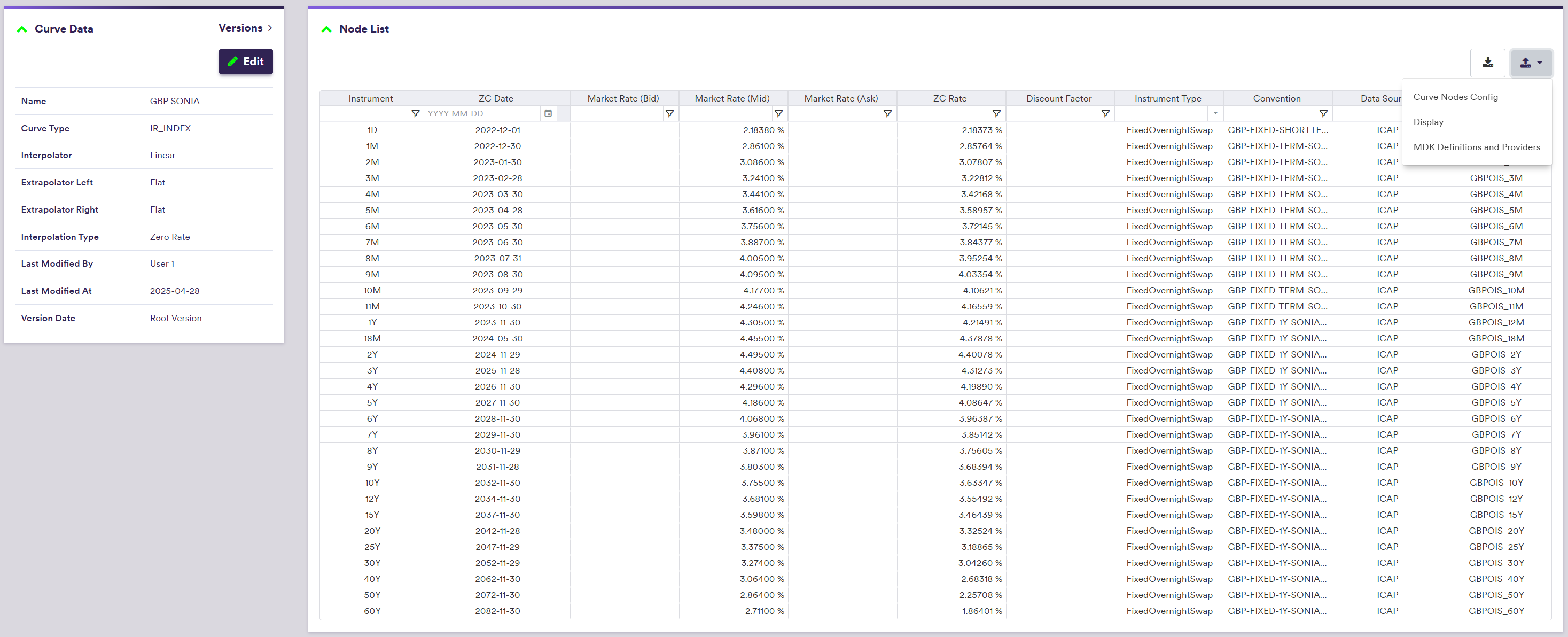
At the interest rate (inflation) curve level, you can view and export the calibrated zero coupon rates (price indices) and discount factors for discount curves.
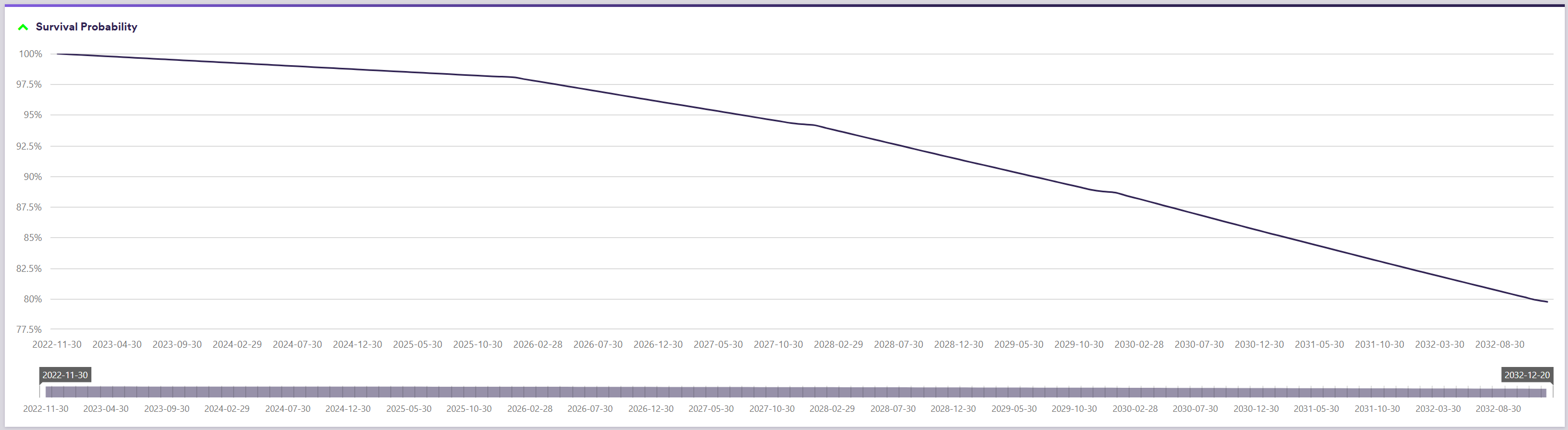
At the credit curve level, you can view and export the calibrated survival probabilities.
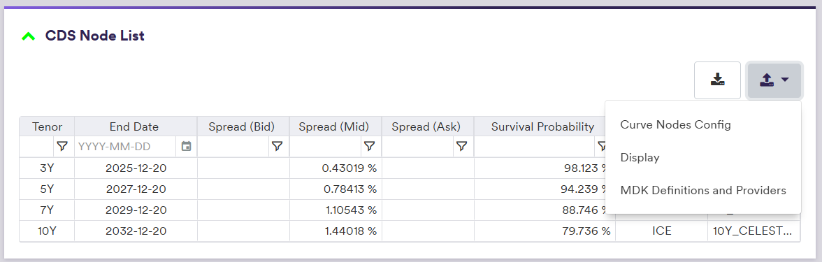
Export Calibration Results
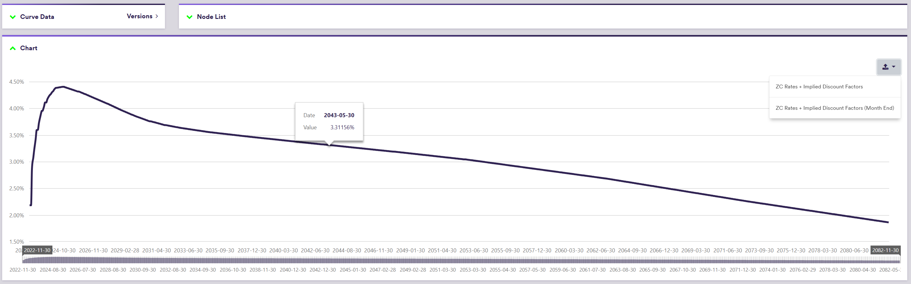
At the curve configuration level (or at the curve level for a single curve), once you have run a curve calibration, you can export calibration results for all curves which have been successfully calibrated, by clicking on (export) and select the required report in the dropdown menu:
- select
Price Indices/ZC/FWD Rates + Implied Discount Factors for data actual curve nodes and monthly interpolated data from the valuation date - select the
[...] (Month End) option for interpolated month end data
The .csv export file will contain the outputs set out in the table below.
| Field Name | |
|---|---|
| Curve Name | The name of the calibrated curve |
| Date | A curve node end date or a date from a monthly schedule starting on the valuation date (associated to an interpolated / implied calibration result). |
| Zero Rate | The (interpolated) calibrated zero coupon rate observed on the Date |
| Price Index | The (interpolated) calibrated inlfation index observed on the Date |
| Forward Rate | The (interpolated) calibrated forward observed on the Date |
| Discount Factor | The implied discount factor derived from the zero coupon rate |
| Market Rate | The (implied) zero coupon inflation market rate corresponding to the price index |
Curve Calibration Algorithm
A curve group may comprise curves that are not all relevant for pricing a given portfolio of trades. Some of the irrelevant curves may be linked to corrupted or missing market data, which in turn could cause the calibration of the whole curve group to fail.
As we want to minimise potential valuation failures, we split the portfolio into sub-portfolios based on various factors such as the trade’s discount currency (*) (**) and each trade leg’s currency (i.e. same or different from the discount currency) to create a non-FX portfolio and an FX portfolio.
We then create a set of sub-curve groups (one per underlying index for the non-FX portfolio and one per foreign currency for the FX portfolio) with the relevant curves for valuation (projection and discount). If these sub-curve groups are successfully calibrated against the prevailing market data, they will be merged into the final calibration curve groups (one for the non-FX portfolio and one for the FX portfolio) used for valuation.
(*) Where Discount Ccy is set to “Local Ccy” instead of a deterministic single currency (e.g USD), user-defined discount currency definition rules will be applied for FX and XCCY trades.
(**) In the absence of an OIS curve in the discount currency in the curve group, the portfolio is first split per explicit underlying index, or per mapped underlying index where applicable, as per user-defined index mapping rules.
Such workflow can be run for illustration purposes at the curve configuration level. As discussed above, it comprises five main steps:
- Portfolio split per discount currency
- Further portfolio split per discount curve
- Further Portfolio split into non-FX vs. FX category
- Sub-curve groups calibration validation
- Sub-curve groups merge and portfolio valuation
We will now discuss each of these steps in detail, and illustrate them with a worked example.
Step 1 - Portfolio split per discount currency
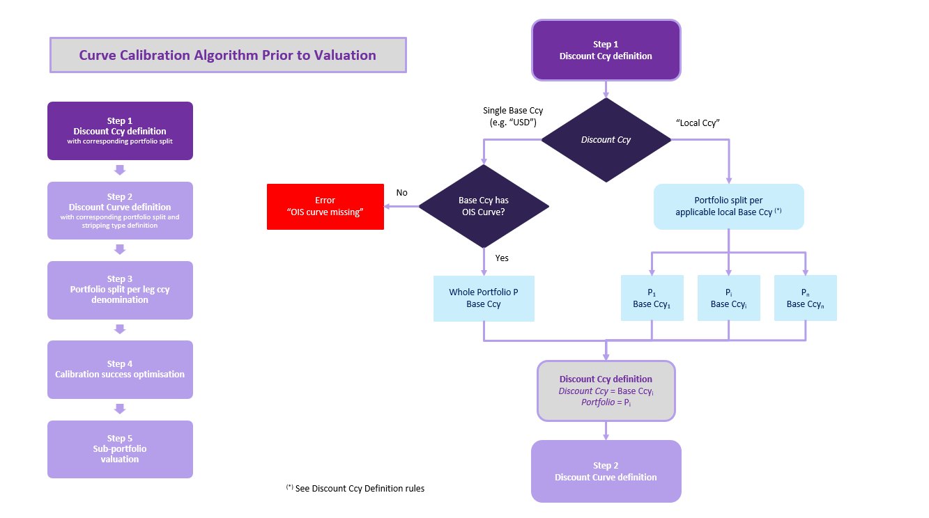
If Discount Ccy is set to a specified single base currency (e.g. USD), no calibration (and thus no valuation) will be performed if there is no OIS curve for such currency in the curve group. The permissible values for a single Discount Ccy are USD, EUR, GBP, AUD, CAD, CHF, JPY, NZD and SGD.
If Discount Ccy is set to “Local Ccy”, the portfolio will be split into sub-portfolios of trades with the same base currency. For single currency trades (e.g. IRS), the base currency will the currency in which both legs are denominated. For FX trades and XCCY trades, this will be determined according to the user-defined discount currency definition rules.
You can refer to our worked example for more details.
Step 2 - Further portfolio split per discount curve
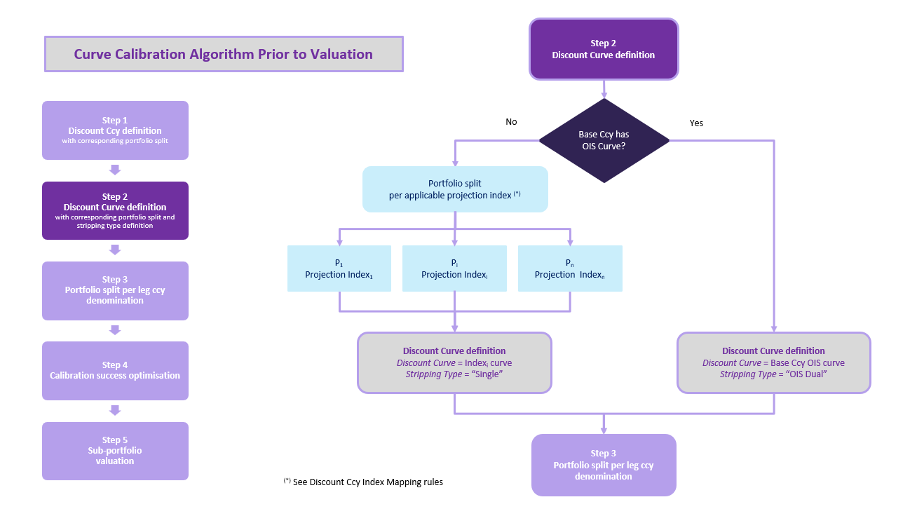
For a given base currency and corresponding sub-portfolio, the curve used to discount cashflows denominated in that base currency will be the associated OIS curve.
If there is no such OIS curve in the curve group, the sub-portfolio will be further split according to the trade’s underlying index, which will be the index linked to the trade (e.g. an IRS trade linked to 3M PLN WIBOR), or in the absence of an explicit underlying index (e.g. in the case of a CDS trade, an inflation trade or an FX trade), the mapped index as per the user-defined index mapping rules. Such index curve will then be used both for discounting and for projection (where applicable).
You can refer to our worked example for more details.
Step 3 - Further portfolio into non-FX vs. FX category
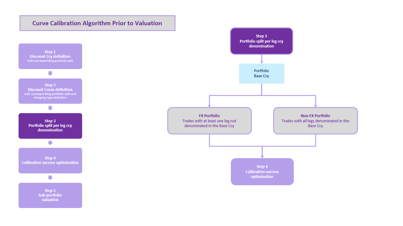
To minimise potential calibration failures, we further split the sub-portfolios into two categories of trades:
- non-FX trades, where both trade legs are denominated in the same currency as the discount currency
- FX trades, where at least one trade leg is denominated in a currency different from the discount currency
We then create two sets of sub-curve groups:
- the first set for the non-FX portfolio containing a sub-curve group (and associated hypothetical sub-portfolio) per underlying index
- the second set for the FX portfolio containing a sub-curve group (and associated hypothetical sub-portfolio) per foreign currency
Each sub-curve group will have the relevant curves for valuation (projection and discount) for all trades in the corresponding hypothetical sub-portfolio.
You can refer to our worked example for more details.
Steps 4 and 5 - Sub-curve groups calibration validation prior to merge and portfolio valuation
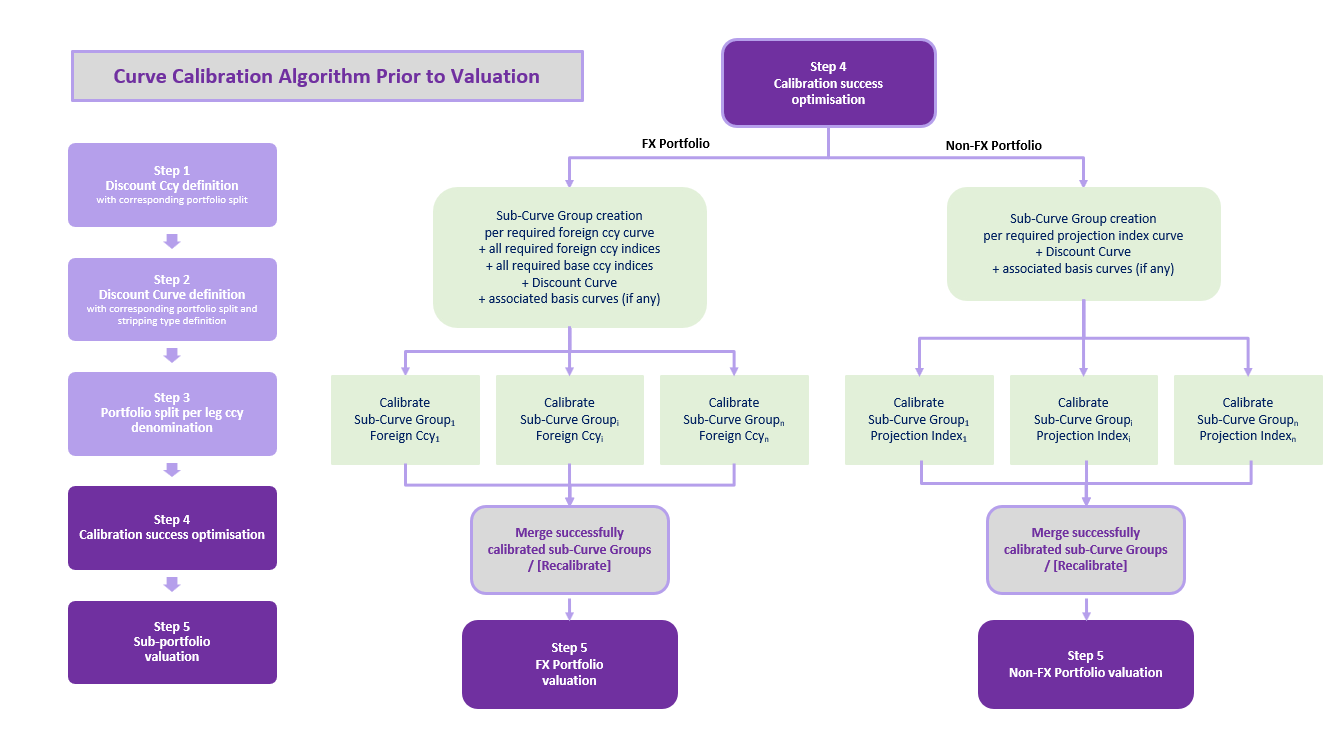
If these sub-curve groups are successfully calibrated against the prevailing market data, they will be merged into the final calibration curve groups used for portfolio valuation, one for the non-FX portfolio and one for the FX portfolio respectively.
You can refer to our worked example for more details.
Worked Example
Let’s take the example of a portfolio comprising the following trades:
- FIX vs EUR ESTR
- FIX vs. EUR 6M EURIBOR
- FIX vs. PLN 3M WIBOR
- FIX vs. PLN 6M WIBOR
- FIX vs. GBP SONIA
- GBP/EUR FX FWD
to be priced with a curve group comprising the following curves:
- EUR ESTR
- GBP SONIA
- EUR 6M EURIBOR
- PLN 3M WIBOR
- PLN 6M WIBOR
- EUR/PLN XCCY curve
- EUR/GBP XCCY curve
- USD/JPY XCCY curve
Case 1: Discount Ccy = “EUR” (single base currency)
Step 1: The portfolio will be valued using EUR as the discount/base currency
Step 2: The portfolio will be valued using EUR ESTR as the discount curve for EUR cashflows
Step 3: The portfolio is split into:
- a non-FX portfolio (comprising the FIX vs. EUR ESTR and the FIX vs. EUR 6M EURIBOR trades)
- an FX portfolio (comprising the FIX vs. PLN 3M WIBOR, FIX vs. PLN 6M WIBOR, the FIX vs. GBP SONIA trades and the GBP/EUR FX FWD trade)
We create two sub-curve groups for the non-FX portfolio, as there are two underlying indexes (EUR ESTR and EUR 6M EURIBOR):
- EUR ESTR index sub-curve group: EUR ESTR curve (discounting and projection)
- EUR 6M EURIBOR index sub-curve group: EUR ESTR (discounting) + EUR 6M EURIBOR curve (projection)
We create two sub-curve groups for the FX portfolio, as there are two foreign currencies (PLN and GBP)
- PNL foreign currency sub-curve group: EUR ESTR (discounting) + EUR/PLN CCY curve (discounting) + PLN 3M WIBOR curve (projection) + PLN 6M WIBOR curve (projection)
- GBP foreign currency sub-curve group: EUR ESTR (discounting) + EUR/GBP CCY curve (discounting) + GBP SONIA curve (projection)
Steps 4 and 5: If there are some bad data points in the EUR 6M EURIBOR curve, the sub-curve group associated with the EUR 6M EURIBOR index will not be calibrated and will not be merged into the final calibration curve group for the non-FX portfolio. As such, only the FIX vs. EUR 6M EURIBOR trade will fail to be value.
If there are some bad data points in the EUR/GBP CCY curve, the sub-curve group associated with the EUR/GBP CCY index will not be calibrated and will not be merged into the final calibration curve group for the FX portfolio. As such, only the FIX vs. GBP SONIA and the GBP/EUR FX FWD trades will both fail to be valued.
If there are some bad data points in the PLN 3M WIBOR curve, the sub-curve group associated with the PLN foreign currency will not be calibrated and will not be merged into the final calibration curve group for the FX portfolio. As such, only the FIX vs. PLN 3M WIBOR and FIX vs. PLN 6M WIBOR trades will both fail to be valued.
Bad data in the USD/JPY XCCY curve will not affect the valuation of the portfolio.
Case 2: Discount Ccy = “Local Ccy” (multiple base currencies)
In our example, there is no OIS curve for PLN in the curve group. Assuming that the FX market pecking order is applied (EUR -> GBP -> AUD -> NZD -> USD -> CAD -> CHF -> JPY -> SGD), the GBP/EUR FX FWD trade will be deemed to be a EUR trade.
Step 1: The portfolio is split into:
- a EUR portfolio (comprising the FIX vs. EUR ESTR trade, the FIX vs. EUR 6M EURIBOR trade and the GBP/EUR FX FWD trade)
- a GBP portfolio (comprising the FIX vs. GBP SONIA trade)
- a PLN portfolio (comprising the FIX vs. PLN 3M WIBOR trade and the FIX vs. PLN 6M WIBOR trade)
Step 2: The discount curves will be as follows:
- the EUR portfolio will be valued using EUR ESTR as the discount curve for EUR cashflows
- the GBP portfolio will be valued using GBP SONIA as the discount curve for GBP cashflows
In the absence of an OIS curve for PLN, the PLN portfolio is further split into two sub-portfolios on an index basis:
- a PLN 3M WIBOR portfolio (comprising the FIX vs. PLN 3M WIBOR trade), which will be valued using PLN 3M WIBOR as the discount curve
- a PLN 6M WIBOR portfolio (comprising the FIX vs. PLN 6M WIBOR trade), which will be valued using PLN 6M WIBOR as the discount curve
Step 3: The EUR portfolio is split into:
- a non-FX EUR portfolio (comprising the FIX vs. EUR ESTR trade and the FIX vs. EUR 6M EURIBOR trade)
- an FX EUR portfolio (comprising the GBP/EUR FX FWD trade)
We create two sub-curve groups for the non-FX EUR portfolio, as there are two underlying indexes (EUR ESTR and EUR 6M EURIBOR):
- EUR ESTR index sub-curve group: EUR ESTR curve (discounting and projection)
- EUR 6M EURIBOR index sub-curve group: EUR ESTR (discounting) + EUR 6M EURIBOR curve (projection)
We create one sub-curve group for the FX EUR portfolio, as there is one foreign currency (GBP):
- GBP foreign currency sub-curve group: EUR ESTR (discounting) + EUR/GBP CCY curve (discounting)
The following sub-curve groups are created for the non-FX GBP, PLN 3M WIBOR and PLN 6M WIBOR sub-portfolios:
- non-FX GBP portfolio sub-curve group: GBP SONIA curve (discounting and projection)
- non-FX PLN 3M WIBOR portfolio sub-curve group: PLN 3M WIBOR curve (discounting and projection)
- non-FX PLN 6M WIBOR portfolio sub-curve group: PLN 6M WIBOR curve (discounting and projection)
Steps 4 and 5: If there are some bad data points in the EUR 6M EURIBOR curve, the sub-curve group associated with the EUR 6M EURIBOR index will not be calibrated and will not be merged into the final calibration curve group for the non-FX EUR portfolio. As such, only the FIX vs. EUR 6M EURIBOR trade will fail to be valued.
If there are some bad data points in the EUR/GBP CCY curve, the sub-curve group associated with the EUR/GBP CCY index will not be calibrated and will not be merged into the final calibration curve group for the FX EUR portfolio. As such, only the GBP/EUR FX FWD trade will fail to be valued.
If there are some bad data points in the PLN 3M WIBOR curve, the sub-curve group associated with the non-FX PLN 3M WIBOR portfolio will not be calibrated, and as such, only the FIX vs. PLN 3M WIBOR trade will fail to be valued.
Bad data in the USD/JPY XCCY curve will not affect the valuation of the portfolio.
CSA Discounting
If CSA Discounting is set to TRUE (see valuation parameters), where a CSA Discount Ccy has been defined at trade level, the portfolio will be split in sub-portfolios of trades with the same CSA Discount Ccy.
Currently, the permissible CSA Discount Ccy values are the same as the permissible values for single Discount Ccy. See permissible discount currency list.
For each CSA Discount Ccy, the corresponding sub-portfolio will be valued using Case 1 above (with Discount Ccy = CSA Discount Ccy).